EM radiation from atoms

Next, we look at how electromagnetic radiation is generated by atoms in materials. We find that the properties of thermal radiation from materials can only be explained with a quantum picture of energy. Then we see that light is also emitted from hot gases in the form of spectral lines, and that the wavelengths of these lines tells us something profound about the nature of atoms.

Thermal radiation

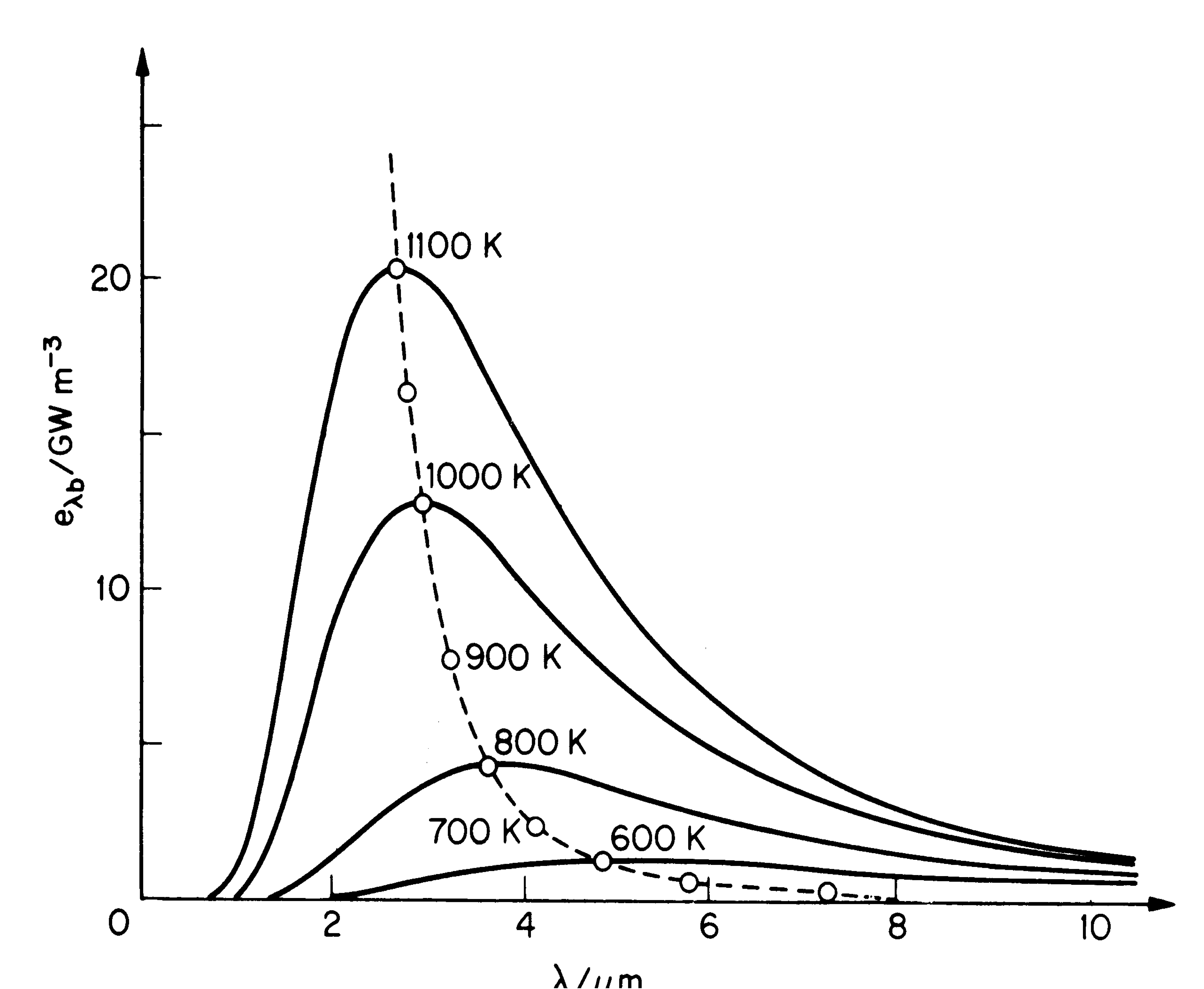
Fig. 5 Wavelength spectrum of thermal radiation at different temperatures.

All materials emit a continuous spectrum of EM radiation when they are at a finite temperature \(T\). This radiation (``thermal radiation” or “black-body radiation”) is observed to obey Stefan’s Law – the power emitted is given by \(P=\sigma A \epsilon T^4,\) where \(A\) is the area of the emitter, \(\epsilon\) is the emissivity (\(=1\) for a perfectly absorbing / black object; \(=0\) for a perfectly reflecting object), and \(\sigma\) is Stefan’s constant \(\sigma = 5.67 \times 10^{-8}\) W m\(^{-2}\) K\(^{-4}\). The intensity distribution of the radiation as a function of wavelength (see Fig. 5) is observed to be zero at short wavelength (\(\lambda \rightarrow 0\)), peaks at some finite wavelength (\(\lambda_p\)), and then falls back to zero as \(\lambda \rightarrow \infty\). Furthermore, \(\lambda_p\) is observed to decrease with increasing temperature according to Wien’s Displacement Law – \(\lambda_p T = 2.9\times 10^{-3}\) m K (a constant).

A classical model of the (continuous) distribution of the wavelengths of standing waves of light inside the emitting material gives the Rayleigh-Jeans formula for the intensity distribution as a function of wavelength:

(5)\[I(\lambda) = \frac{2\pi c k_B T}{\lambda^4},\]

where \(k_B\) is Boltzmann’s constant. This distribution diverges to infinity as \(\lambda \rightarrow 0\) (the ultra-violet end of the visible light spectrum) however, and does not peak at any finite wavelength, in contrast to what is observed. This is the “Ultraviolet Catastrophe” of classical physics.

The solution to the Ultraviolet Catastrophe is obtained by assuming that rather than a continuous distribution of wavelengths only a discrete set of wavelengths (modes) is allowed, of energy \(E=nhc/\lambda\), where \(n\) is an integer and \(h\) is Planck’s constant. This gives rise to the Planck formula for the intensity distribution as a function of wavelength:

(6)\[I(\lambda) = \frac{2\pi h c^2}{\lambda^5\left(e^{hc/\lambda k_B T}-1\right)},\]

where \(c\) is the speed of light. This is the power radiated per unit area per unit wavelength. This formula indeed gives a distribution that peaks at a finite wavelength that depends on \(T\) consistently with Wien’s displacement law. Furthermore, when \(\lambda \gg hc/k_B T\) this formula can be approximated by the Rayleigh-Jeans formula, so the quantum physics result is consistent with the classical picture at long wavelength and low energy.

Example 2.1

Question

To a good approximation, the sun’s surface is a blackbody with a surface temperature of 5800 K. Find the approximate power per unit area radiated from the sun’s surface in the wavelength range 600.0 to 605.0 nm.

Solution

The wavelength range is small compared with the mean wavelength \(\lambda = 602.5\) nm. We can therefore assume this value for the wavelength, with a small range of wavelength \(\Delta \lambda = 5.0\) nm. We use the Planck formula for the intensity distribution (i.e. power per unit area per unit wavelength) (Eqn. (6)) as a function of wavelength and multiply by the wavelength range to get \(I(\lambda)\Delta\lambda = 3.9 \times 10^5\) W m\(^{-2}\).

Line spectra

When observing EM radiation emission from very hot gases we see additional features in the emission spectrum compared with hot solid materials. Overlaying the thermal radiation distribution we see sharp peaks of “lines” in the emission spectrum, that are characteristic of the atoms that are in the gas. To understand these emission lines we need to understand the structure of the atoms in the gas.

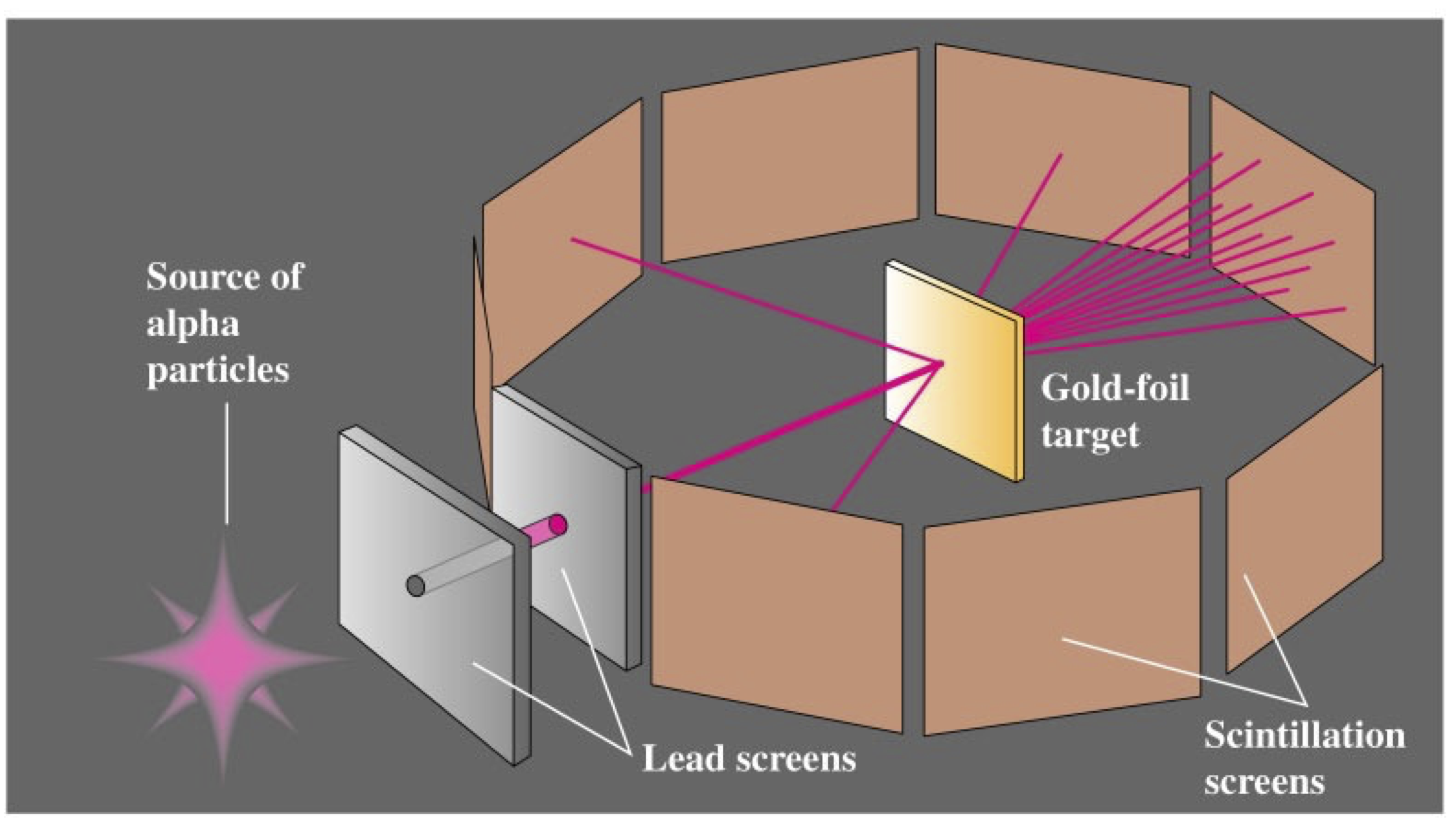
Fig. 6 The Rutherford scattering experiment.

Since electrons were discovered by Thomson in 1897, we have known that atoms are partly composed of negatively charged electrons. Given that atoms are neutral, we also know that there must be a balancing positive charge in the atoms. In the “plum pudding model” of the atom, the electrons are scattered randomly through a positively charged material. The Rutherford scattering experiment (see Fig. 6) demonstrates that this picture is incorrect however. In this experiment a collimated beam of energetic, positively charged \(\alpha\) particles is fired at a thin foil of gold. The gold foil is surrounded by scintillator screens, which emit a flash of light whenever they are hit by an \(\alpha\) particle. Most \(\alpha\) particles are observed to pass straight through the foil, or are deflected through only very small angles. However, occasionally an \(\alpha\) particle is deflected through a very large angle, possibly as large as 180\(^\circ\).

The explanation of the results seen in the Rutherford scattering experiment is that the mass distribution in the atoms is not uniform, as in the plum pudding model, but rather consists of a small, dense, positively charged “nucleus”, surrounded by a diffuse cloud of light, negatively charged electrons. The \(\alpha\) particles mostly pass straight through the diffuse electron cloud and hence are not deflected. However, occasionally they strike a heavy nucleus head-on, in which case they can be deflected through large angles.

The wavelengths of the emission lines from Hydrogen, and some alkali metals, are observed to empirically follow the Rydberg-Ritz formula:

(7)\[\frac{1}{\lambda} = R\left(\frac{1}{n_2^2} - \frac{1}{n_1^2}\right),\]

where \(n_2\) and \(n_1\) are integers, \(n_2 < n_1\), and \(R= 1.097776\times 10^7\) m\(^{-1}\) is the empirically measured “Rydberg constant”. In order to understand the origin of this formula we can use our knowledge of the structure of the atom from the Rutherford scattering experiment. Given that the negatively charged electrons surround heavy positively charged nuclei it is natural to consider a “planetary” model (or “Rutherford model”) of the Hydrogen atom, in which each electron orbits a nucleus, with the electrostatic attraction between the nucleus and the electron providing the centripetal force of the orbit:

(8)\[\frac{Ze^2}{4\pi \epsilon_0 r^2} = \frac{m_ev^2}{r}, \label{eqn:centrip}\]

where \(Z=1\) is the charge on the Hydrogen nucleus, \(r\) is the radius of the orbit and \(v\) is the electron velocity.

We can now calculate the total energy of an electron orbiting the Hydrogen nucleus. It is the sum of its kinetic energy \(E_K = (1/2) m_e v^2\) and electrostatic potential energy \(E_U = -Ze^2/4\pi\epsilon_0 r\) (remembering the charge on an electron is \(-e\)). The kinetic energy can be evaluated by multiplying both sides of Eqn. (8) by \(r/2\) to obtain

(9)\[E_K = \frac{Ze^2}{8\pi\epsilon_0 r}. \label{eqn:ek} \]

The total energy is then:

(10)\[E_{\rm tot} = E_K + E_U = -\frac{Ze^2}{8\pi\epsilon_0 r}.\]

Setting \(Z=1\), this is the energy of the electron according the Rutherford model of the Hydrogen atom.

This leaves a couple of problems however. Firstly, although this tells us the energy of the electron in terms of its orbital radius \(r\), we do not know what values \(r\) should take. Secondly, according to classical electromagnetism an accelerating charge continuously emits electromagnetic radiation and hence loses energy. The direction of the velocity of the orbiting electron is changing, even if its speed is not, and hence the electron is accelerating in its orbit. The electron should therefore lose energy by radiation and the orbit should decay, with the electron spiralling into the nucleus. The atom should therefore not be stable.

The Bohr model of the atom

Bohr resolved this apparent paradox by proposing three new postulates:

1. Only certain electron orbits (``stationary states”) are allowed, and in those orbits the electron does not emit em radiation.

2. An atom emits radiation only when an electron makes a transition from one stationary state to another.

3. The frequency of the radiation emitted when an electron makes a transition from one stationary state with energy \(E_1\) to one with energy \(E_2\) is given by \(f = (E_1 - E_2)/h\), where \(h\) is Planck’s constant.

Now, if an electron moves from an orbit of radius \(r_1\) and energy \(E_1\) to a second orbit of smaller radius \(r_2\) and energy \(E_2\) then according to the Rutherford model the difference in energies (and hence the energy of the emitted radiation) is given by

(11)\[\Delta E = E_1 - E_2 = -\frac{e^2}{8\pi\epsilon_0 r_1} - -\frac{e^2}{8\pi\epsilon_0 r_2} = \frac{e^2}{8\pi\epsilon_0 }\left(\frac{1}{r_2} - \frac{1}{r_1}\right).\]

According to Bohr’s third postulate this must be equal to \(hf\), i.e. Planck’s constant times the frequency of the emitted radiation.

We now need to calculate the radii of the allowed stationary state electron orbits. Bohr made a fourth assumption at this point, which is that the magnitude of the angular momentum of the electrons is quantised – in other words that it can only take on discrete values (we shall see why later). The magnitude of the angular momentum is given by \(L = pr = m_evr\), where \(p\) is the linear momentum of the electron. Bohr set this equal to an integer multiple of \(\hbar=h/2\pi\), so that \(m_evr = n\hbar.\) We can now rearrange this equation to get an expression for \(v^2\) and set that equal to a similar expression obtained by rearranging Eqn. (9) (with \(Z=1\) for Hydrogen):

(12)\[v^2 = \frac{n^2\hbar^2}{m_e^2r^2} = \frac{e^2}{4\pi \epsilon_0 m_e r}.\]

Rearranging this we find finally that

(13)\[r = \frac{n^2\hbar^24\pi\epsilon_0}{m_e e^2}=\frac{n^2 h^2 \epsilon_0}{\pi m_e e^2}=n^2 a_0,\]

where, in the last step, we have introduced \(a_0\) as the radius of the smallest (\(n=1\)) orbit of the hydrogen atom: \(a_0 = h^2 \epsilon_0/\pi m_e e^2\).

We can substitute this expression for the radii of the stationary states into the formula for the energy loss \(\Delta E\) of an electron moving between orbits of radius \(r_1\) and \(r_2\) and use Bohr’s third postulate to obtain

(14)\[f = \frac{e^2}{8\pi\epsilon_0 h}\left(\frac{1}{r_2} - \frac{1}{r_1}\right) = \frac{e^2}{8\pi\epsilon_0 ha_0}\left(\frac{1}{n_2^2} - \frac{1}{n_1^2}\right) = \frac{e^4 m_e}{8\epsilon_0^2 h^3}\left(\frac{1}{n_2^2} - \frac{1}{n_1^2}\right).\]

Comparing this with the Rydberg-Ritz formula for \(1/\lambda\) and remembering that \(f=c/\lambda\) we find that the constants multiplying the bracket in this expression should equal the empirical Rydberg constant times the speed of light \(c\). In fact the agreement is excellent, confirming that Bohr’s postulates applied to the Rutherford model (now called the “Bohr model”) provide an explanation for the Rydberg-Ritz formula.

Unfortunately, the Bohr model does not provide a complete description of atomic physics. In particular it:

• does not work well for many-electron atoms (even helium);

• cannot explain the fine structure of spectral lines observed at high resolution, or relative intensities of spectral lines;

• cannot explain the effect of magnetic fields on spectral lines (the Zeeman effect);

• is fundamentally inconsistent with Heisenberg’s uncertainty principle (see Topic 5).

To resolve these problems we need a fundamentally different approach to quantum physics – quantum mechanics (Topic 4). First, though, we need to understand why the angular momentum of electrons should be quantised.

Example 2.2

Question

Find the total energy of an electron in (a) the ground state and (b) the first excited state of a hydrogen atom. What is the wavelength of a photon emitted when an electron undergoes a transition from the first excited state to the ground state?

Solution

We can substitute the expression for the orbital radius from Eqn. (13) into the expression for the total energy of the electron Eqn. (10), with \(Z=1\) for hydrogen. This gives \(E_n = -13.6\) \(e\)V \(/n^2\), where \(n\) is the principal quantum number. The total energies are then (a) \(E_1 = -13.60\) \(e\)V for the ground state (\(n=1\)) and (b) \(E_2 = -3.40\) \(e\)V for the first excited state (\(n=2\)). The energy of the emitted photon is equal to the difference between the total energies of the two levels and is then \(\Delta E = E_2-E_1 = 10.20\) \(e\)V. Using \(\Delta E=hc/\lambda\), and hence \(\lambda = hc/\Delta E\), we find that \(\lambda = 122\) nm. We could also obtain this result more directly from Eqn. (14)